lastmod: 11 May, 2020
# general use
library(tidyverse)
library(here)
library(readxl)
library(reshape2)
# process text
library(tm)
library(tidytext)
library(wordcloud)
# graphics
library(ggplot2)
# output
library(flextable)
Introduction
I will not present here all
Rcode used in the analysis, but rather only code pertaining to the text analysis. Less relevant code (e.g., table viewing, formatting, etc. is ignored).
The data used here comes from students’ responses to an academic task that required them to present a project of their choice, describe that project and talk about its importance, and peform a SWOT analysis on the said project. In addition, as an alternative choice, students described their understanding of ‘cognitive biases’.
The graphs below give us a walkthrough the most frequent concepts that visited my students minds when asked about their projects and their projects’ importance, as well as the positive or negative affects accompanying their written expression…
However, when reading/interpreting it, remember that there were only 60 responses, and thus, a rather small volume of data to work with.
> Note: due to privacy implications, the source data file is made available only on request and under special restrictions
>
The table below shows that the fields associated with the students’ projects have the highest number of responses (60) whereas the field for cognitive biases has a rather small number of responses.
# calculate number of responses per column in original raw data file
df_raw %>%
  dplyr::select(-c(`Motivatie / Reason`, "Timestamp", "RespID")) %>%
  dplyr::filter(`Limba cursului / Course language` == "Engleza / English") %>%
  map_df(., ~ length(which(!is.na(.)))) %>%
  t() %>%
  as.data.frame() %>%
  rownames_to_column() %>%
  flextable::flextable() %>%
  flextable::set_header_labels(rowname = "Field", V1 = "Number of responses") %>%
  flextable::bold(part = "header") %>%
  flextable::align(align = "left", part = "all") %>%
  flextable::fontsize(size = 11) %>%
  flextable::font(fontname = "Open Sans", part = "all") %>%
  flextable::autofit()
Field | Number of responses |
Limba cursului / Course language | 70 |
Descrierea proiectului / Description of your project | 60 |
Importanta proiectului / Significance of the project | 60 |
S (puncte tari / strengths) | 60 |
W (puncte slabe / weaknesses) | 60 |
O (oportunitati / opportunities) | 60 |
T (amenintari / threats) | 60 |
Text sarcina 4 / Text assignment 4 | 8 |
Not all data collected through this assignment is relevant for our analysis here. Our main purpose for this example is to extract some meaningul information about recurring themes in students responses. To this end, we need to identify those fields that contain enough responses for a fruitful ’bag-of-words (Brownlee, 2017; Wikipedia, n.d.). Inspecting the table above, it appears that the most promising field could be the project description with 60 total answers.
# create data frame for EN responses and rename columns for easier use
df_raw_en <- df_raw %>% setNames(c("TS", "ID", "LANG", "DESCR", "IMP", "S", "W", "O", "T", "MOT", "T4"))
# select only data from EN respondents by filtering out non-English responses
df_raw_en <- df_raw_en %>% dplyr::filter(LANG == "Engleza / English")
The step-by-step approach
It’s perhaps best to start with a step-by-step, more hands-on approach, which can give us a sense of the procedures involved in preparing the text for data visualization. To this end we use the functions of the tm package (Feinerer, Hornik, & Meyer, 2008). The disadvantage is you use more commands until you reach the final word bag. However, it may more useful for beginners because it takes you step by step through the process of getting the word bag.
If you only want to see how all responses at once, concatenated, you can use the cat command from base R.
# the chunk option results='hide' hides the output, otherwise we'd have a very long reading to do...
# create word corpora ----
# word corpus for <description>
df_corpus_descr <- df_raw_en %>% dplyr::select(c("ID", "DESCR")) %>% dplyr::filter(!is.na(DESCR))

# word corpus for <importance>
df_corpus_imp <- df_raw_en %>% dplyr::select(c("ID", "IMP")) %>% dplyr::filter(!is.na(IMP))

# # view word corpora for project <description>
# df_corpus_descr[2] %>% unlist() %>% cat()
However, we’re interested in doing some modifications to the text, consisting in removing punctuation signs, converting all words to lower case, removing so-called ‘stop words’, i.e., words without specific meaning, like connecting words (e.g., and, if, etc.). Note: I used sequential numbering for successive transformations on the same corpus so that each partial output can be viewed separately as we progress through each step.
#
# put all responses from the column DESCR into a single list
df_corpus_descr_tm_txt_1 <- paste(as.list(df_corpus_descr$DESCR))
# create a corpus from vector source
df_corpus_descr_tm_txt_2 <- Corpus(VectorSource(df_corpus_descr_tm_txt_1))
# convert any capitalized word to lower case
df_corpus_descr_tm_txt_3 <- tm_map(df_corpus_descr_tm_txt_2, tolower)
# remove punctuation
df_corpus_descr_tm_txt_4 <- tm_map(df_corpus_descr_tm_txt_3, removePunctuation)
# remove extra white spaces
df_corpus_descr_tm_txt_5 <- tm_map(df_corpus_descr_tm_txt_4, stripWhitespace)
# the stop words can be viewed with
# head(stopwords("en"))
# remove stop words
df_corpus_descr_tm_txt_6 <- tm_map(df_corpus_descr_tm_txt_5, removeWords, stopwords("en"))
# view various stages of text processing
df_corpus_descr_tm_txt_1 %>% cat()              # original corpus
df_corpus_descr_tm_txt_2 %>% unlist() %>% cat() # original corpus as list
df_corpus_descr_tm_txt_3 %>% unlist() %>% cat() # lower case
df_corpus_descr_tm_txt_4 %>% unlist() %>% cat() # remove punctuation
df_corpus_descr_tm_txt_5 %>% unlist() %>% cat() # strip white space
df_corpus_descr_tm_txt_6 %>% unlist() %>% cat() # remove stopwords
The sequence of commands above concludes a sort of data preprocessing for our source of words. Now, we need to go to a deeper level of processing, consisting in placing the source into a container more suited for this analysis with tm. That specific container is a matrix of words per each document containing responses (remember, we started with 60 responses).
# create a document term matrix
dtm <- DocumentTermMatrix(df_corpus_descr_tm_txt_6)
dtm <- as.matrix(dtm)
# transpose the DTM for easier vieweing (words on rows and source responses as columns)
dtm <- t(dtm)
A popular use for these kind of matrices is building word clouds. In order to do that, we’ll use the wordcloud function from the wordcloud package,
# compute number of occurences of each word
n_occur <- rowSums(dtm) %>% sort( . , decreasing = TRUE)
# create a word cloud from the first 100 most frequent terms in students' responses
wordcloud(names(head(n_occur,100)), head(n_occur,100), scale=c(2,1))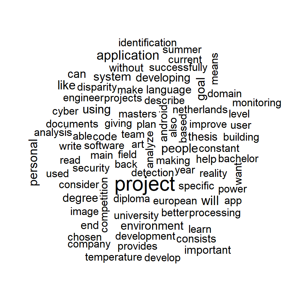
Since the word ‘project’ is the actual name of the students’ task, it is obviously overly favored in a biased way with respect to other words. Hence, it may be more relevant to build the word cloud without it.
trim_n_occur <- n_occur[-1]
wordcloud(names(head(trim_n_occur,100)), head(trim_n_occur,100), scale=c(2,1))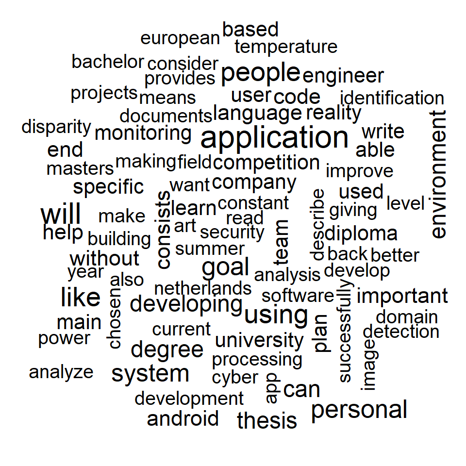
A more ‘expert’ approach
If the approach before showed us how to process the data step-by-step, more experienced user can make use of another package, i.e., the tidytext package(Silge & Robinson, 2016), whose functions are a bit more esoteric, in the sense they’re more opaque as to what each function does, and requires deeper knowledge about what processes like ‘tokenization’ mean. .
# create word corpora ----
# word corpus for <description>
df_corpus_descr <- df_raw_en %>% dplyr::select(c("ID", "DESCR")) %>% dplyr::filter(!is.na(DESCR))
# word corpus for <importance>
df_corpus_imp <- df_raw_en %>% dplyr::select(c("ID", "IMP")) %>% dplyr::filter(!is.na(IMP))
# tokenize the corpus text ----
# for <description>
tidy_corpus_descr <- df_corpus_descr %>%
tidytext::unnest_tokens(. , input = "DESCR" , output = "word")
# for <importance>
tidy_corpus_imp <- df_corpus_imp %>%
tidytext::unnest_tokens(. , input = "IMP" , output = "word")
# remove the stop words ----
# for <description>
clean_tidy_corpus_descr <- tidy_corpus_descr %>% anti_join(stop_words)
# for <importance>
clean_tidy_corpus_imp <- tidy_corpus_imp %>% anti_join(stop_words)Visualization of constructs and sentiments
frequency of most common constructs in the projects’ descriptions
Our people really like their application, and, surprisingly, coming strong on second place, they’re pretty concerned with other people. Fear not, though, they recover with personal in third place…
# graph most common words

clean_tidy_corpus_descr %>%
  count(word, sort = TRUE) %>%
  filter(n > 5 & n < 30) %>%
  mutate(word = reorder(word, n)) %>%
  ggplot(aes(word, n)) +
  geom_col() +
  coord_flip() +
  scale_color_brewer(palette = "Dark2")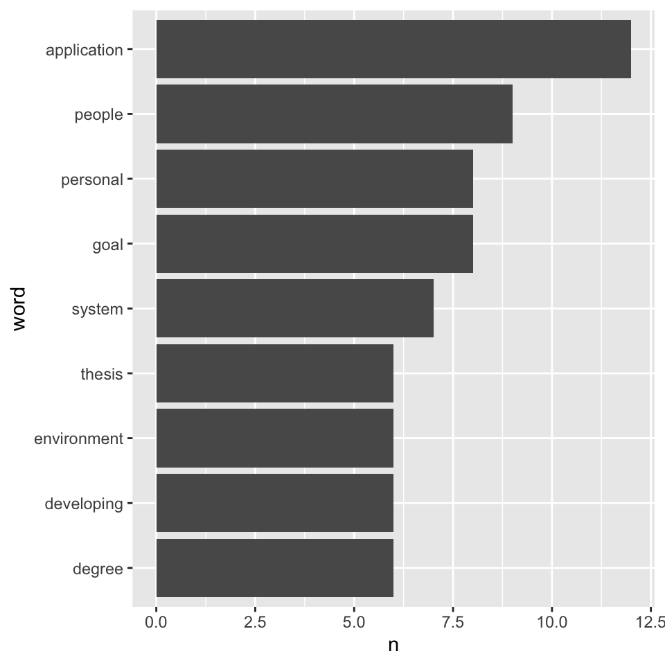
word cloud constructs in the projects’ descriptions
This is pretty much the same thing as above, just in another shape
clean_tidy_corpus_descr %>% filter(word != "project") %>% count(word) %>% with(wordcloud(word, n, max.words = 100))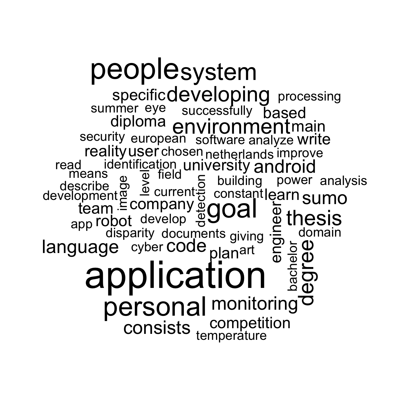
sentiments in the project
The word cloud separated by sentiment type, below, is not humongously illustrative, but it does show what postivies our students value most and what they fear most.
Again, be mindful when interpreting it. For instance, ‘master’ here does not refer directly to mastering something, alas, but rather to the students’ intention to pursue masters courses. In the same vein, the term
clean_tidy_corpus_descr %>%
  inner_join(get_sentiments("bing")) %>%
  count(word, sentiment, sort=TRUE) %>%
  acast(word ~ sentiment, value.var = "n", fill = 0) %>%
  comparison.cloud(colors = c("gold3", "green"))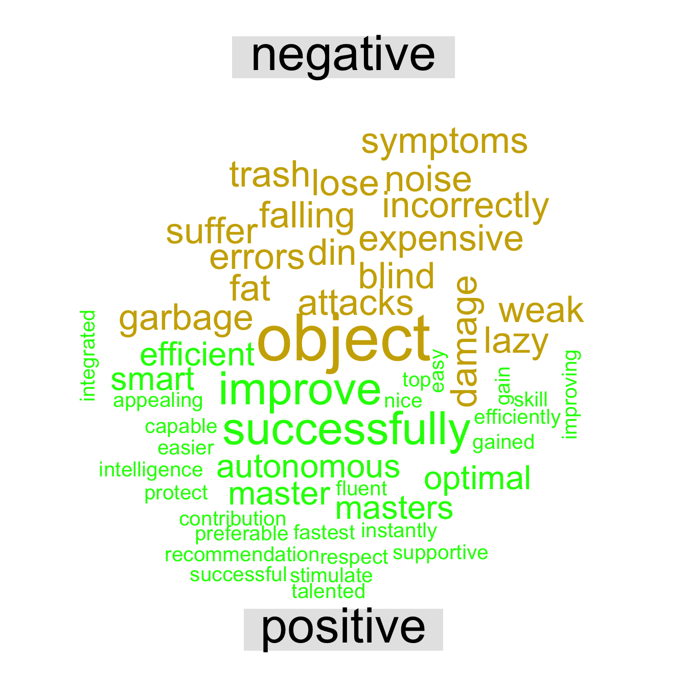
Useful readings
A Light Introduction to Text Analysis in R. (2019). Medium. Retrieved 25 October 2019, from https://towardsdatascience.com/a-light-introduction-to-text-analysis-in-r-ea291a9865a8
Robinson, J. (2019). Text Mining with R. Tidytextmining.com. Retrieved 25 October 2019, from https://www.tidytextmining.com/
Wikipedia. (n.d.). Bag-of-words model. https://en.wikipedia.org/wiki/Bag-of-words_model
References
Brownlee, J. (2017, October). A gentle introduction to the bag-of-words model. https://machinelearningmastery.com/gentle-introduction-bag-words-model/.
Feinerer, I., Hornik, K., & Meyer, D. (2008). Text mining infrastructure in r. Journal of Statistical Software, 25(5), 1–54. Retrieved from http://www.jstatsoft.org/v25/i05/
Silge, J., & Robinson, D. (2016). Tidytext: Text mining and analysis using tidy data principles in r. JOSS, 1(3), 37. https://doi.org/10.21105/joss.00037
Wikipedia. (n.d.). Bag-of-words model. https://en.wikipedia.org/wiki/Bag-of-words_model.
Last modified on 2021-04-07