A brief intro on scripts and libraries

This is rather important post. And, it is also the last of the introductory posts. It introduces the scripts and the libraries/packages and it provides a first example of using them. I believe it makes more sense if we introduce them with a practical example, for a specific task and with a specific goal.

Scripts

Until now, we’ve used the Console to write our commands. This is perfectly fine and doable, and as I said, we’ll soon feel the need to use it again, because there are plenty of times when it is needed.
Still, the main reason for using R is to have a history of our work. A ‘program’ that we can adjust, expand, modify, optimize, as we progress with our data processing and analyses.

Libraries

‘Libraries’ or ‘packages’ are the R’s equivallent of menu ‘commands’ in other statistical software.

In IBM’s SPSS^TM (IBM Corp., 2017), which is a point-and-click or command-menu type of software, one does the analyses and gives the commands by identifying the proper menu, selecting the adequate command, and then navigating the corresponding dialog box.

For instance, you may want to graph a scatterplot. Specifically, one goes to the ‘Graphs’ menu, chooses ‘Legacy Dialogs’ and then ‘Scatter/Dot’, which opens up the ‘Scatter/Dot’ dialoag box, with several options for building a scatterplot.

In R, one does this by writing the appropriate command for getting a scatterplot of the pair of variables of interest. We’ll do that, together, in a jiffy.

Using scripts and libraries, finally…

Your first script

Look up to the File menu, click it, and identify the submenu ‘New File’. Hover/click on it an it opens a list of new types of files that you could open/create. Select ‘R script’ (or, alternatively, if you like using keyboard shortcuts, ignore everything and just click ‘CTRL+SHIFT+N’).

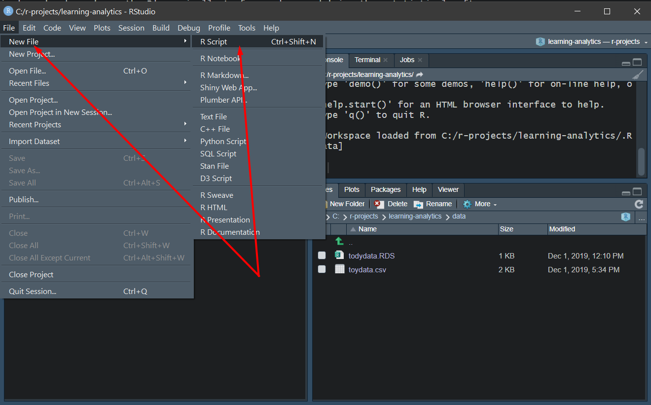
Fig. 1: Use the File>New File>R Script menu commands to create a new R script (or use CTR+SHIFT+N to the same effect)

Now, almost as important as creating your script is to save it… Please, remember to save your files often. R Studio has a sort of a build in protection to accidentally closing your files or projects, but don’t rely on that. Get into the habbit of always knowing what your files’ status is and everytime you make some substantial progress, save them. This is no different than working with any other software or any other project. This is good practice regardless if your write your Word report, do your calculations in Excel, or write a lenghty email memo.

Use ‘CTR+S’ from within the open script window or use the save icon under the title of your window, or go the menu ‘File’ and choose ‘Save’ (or ‘Save as…’ if you want to save your file with a different name).

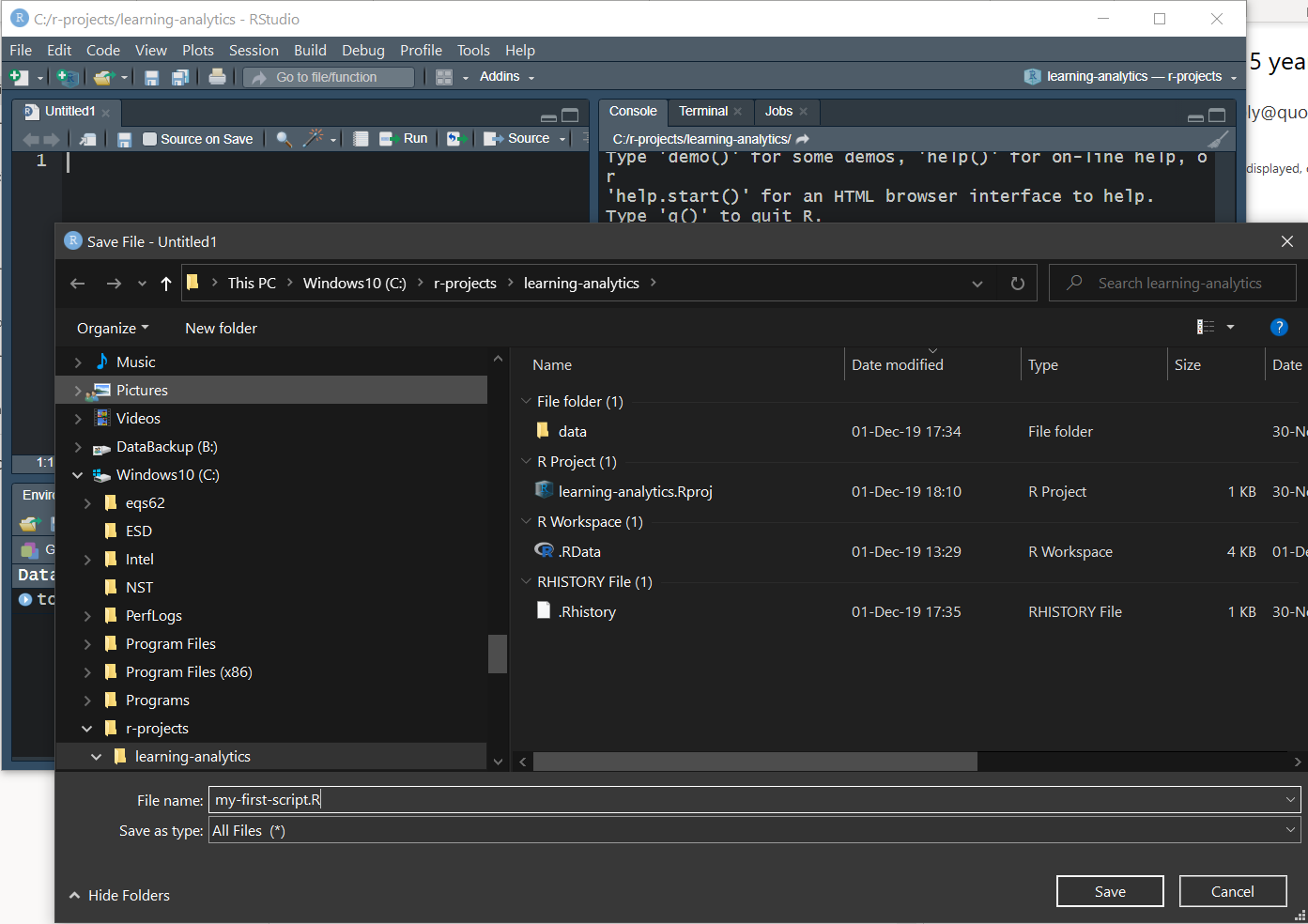
Fig. 2: Save your file!

And now, you have your very own first script. Empty as it is, it yours to do as you please. My suggestion is to use it to get to know what libraries, or packages, are.

Get some action in our first script. What about that scatterplot…

Earlier in this post, I brought up the scenario of doing a scatterplot. We already have some data that we can use to this end.

# use the variables cweight and cheight from the 'toydata' file to draw our first scatterplot 
plot(toydata$cheight, toydata$cweight)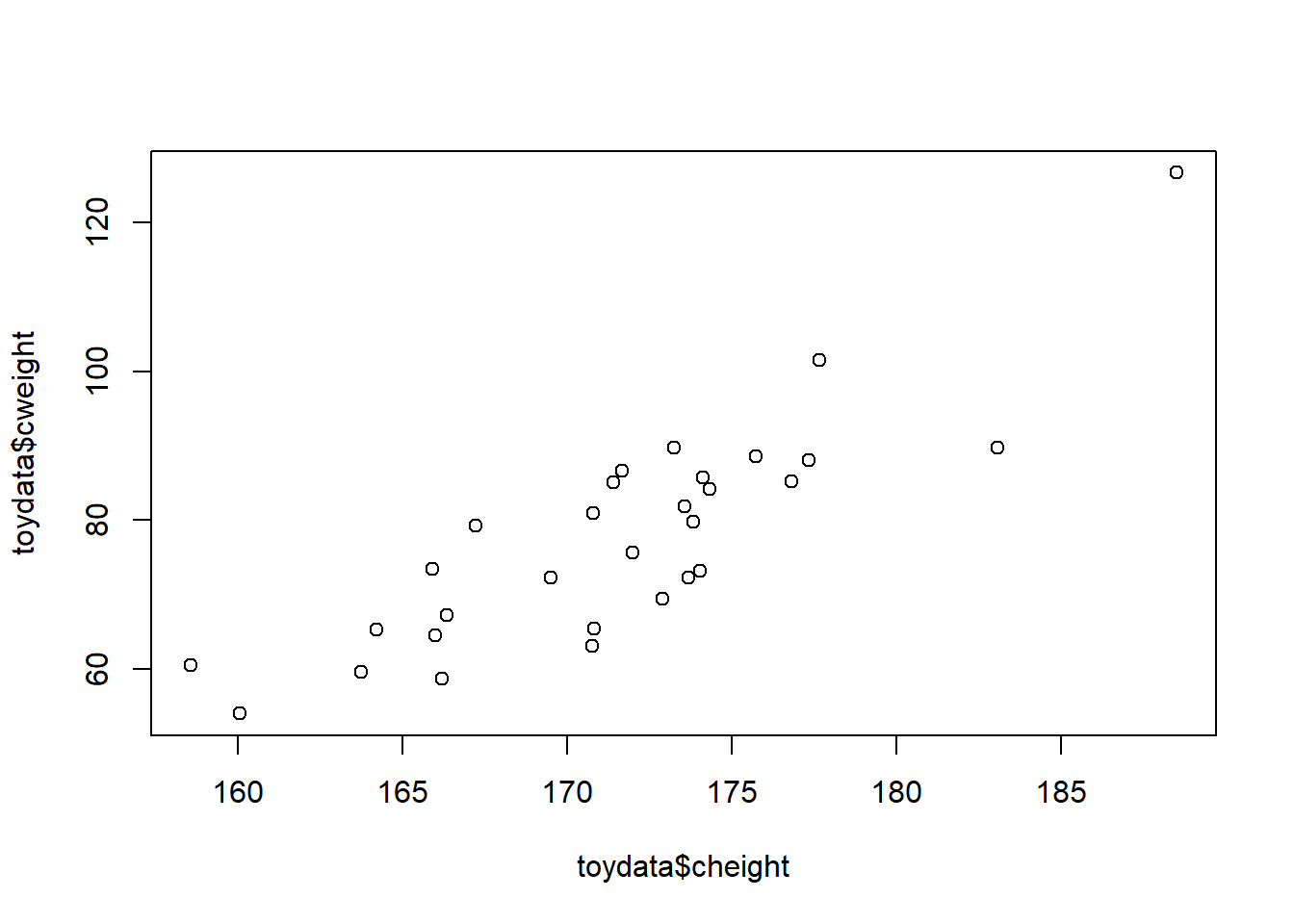

And we can further cosmetize this

plot(toydata$cheight, toydata$cweight,
     xlab = "Height", 
     ylab = "Weight",
     pch = 19)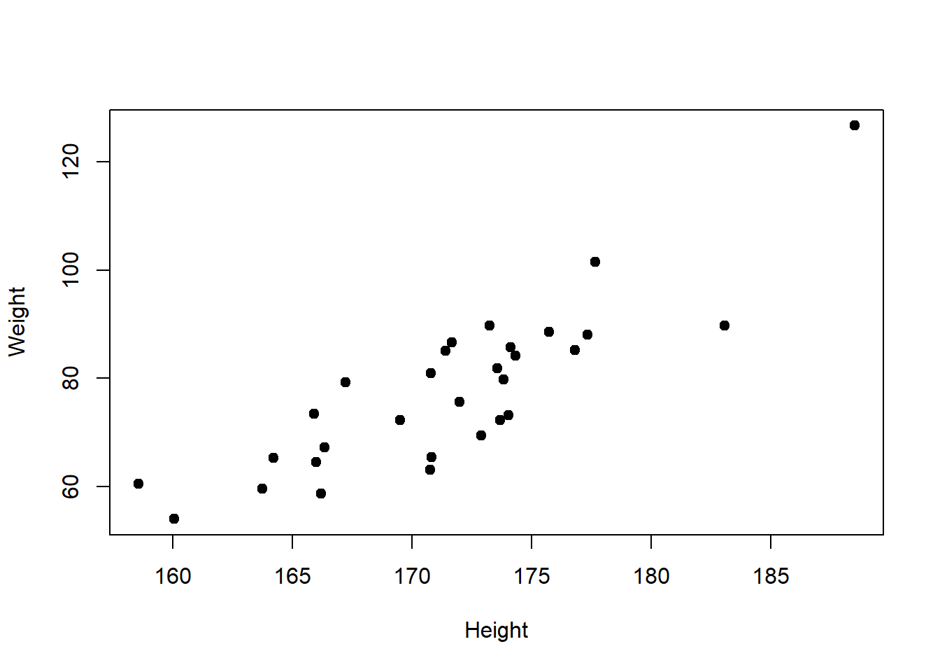

Bring up those libraries, already…

I also said in the beginning that this post will be, among others, about using the ‘libraries’, or ‘packages’ as they are also called. And this is what we’ve been building up to, until now.

Somehow, we didn’t need (only apparently so) any libraries to do it. That only appears so, because we’ve used R’s build in libraries, with no need to specifically call for a dedicated library.

So, let us use our first libraries. The above graph was done using R’s own build in capabilities, but as we’ll see, when things get more complicated and we’re in need of more complex and more refined analyses and graphs.

We’ll rebuild this graph, but this time we’ll use a dedicated library, to do so. It’s nothing less than Hadley Wickham’s famous ‘plot2’ (Wickham, 2016) (we’ll also use other packages from the ‘tidyverse’ (Wickham et al., 2019) collection).

Before we can use ‘ggplot2’, we need to install it.

# install 'ggplot2' in case it isn't already in your packages library (and it shouldn't be, if you're a new user of R and R Studio)
install.packages("ggplot2")

Alternatively, if you’re unsure if your required library/package is already installed in your system, but you can’t remember, you can use the script below, which only installs the package if you need to.

# install the required package/library if not already installed 
if (!require(ggplot2)){
        install.packages(ggplot2)
}

We are now ready to use ‘ggplot2’.

# load the 'ggplot2' library that we'll be using to rebuild our scatter plot
library(ggplot2)

# use ggplot2 to command the graphing of a scatter plot
ggplot(data = toydata, aes(x = cheight, y = cweight)) + geom_point()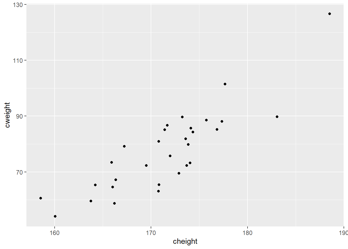

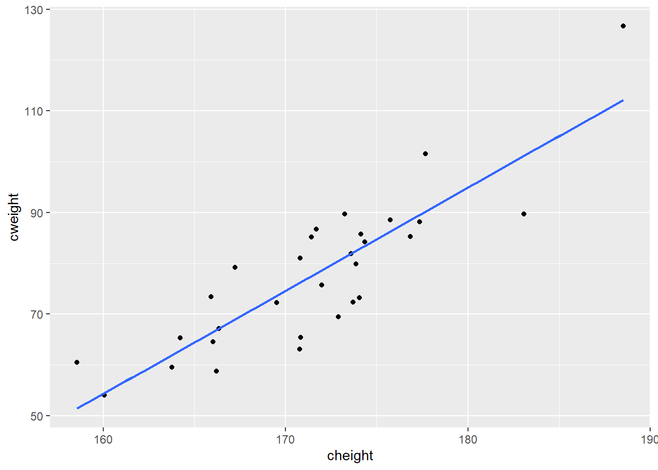
And here it is, a scatter plot made using ‘ggplot2’, a specially dedicated library with amazing graphical capabilities. Will cosmetize it a bit more, just because we can, but our point about using a special library was made. It case it was not obvious from the command we wrote, ‘library(ggplot2)’ was the command that loaded the ‘ggplot2’ library into our system.

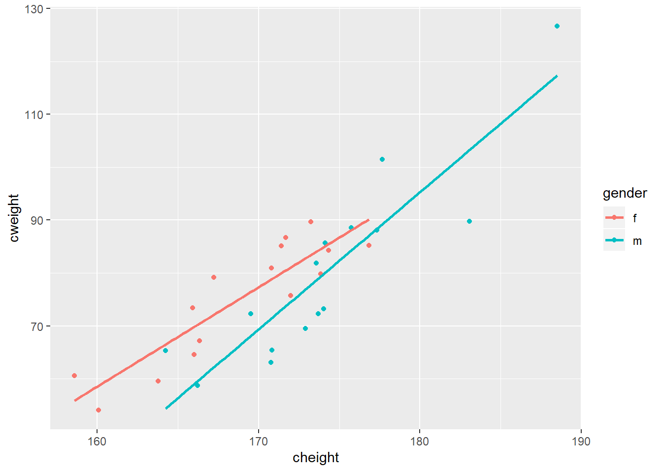
And we can even add a color separation for gender:

Now, before we get carried away, let’s remember that our main purpose here, in this post, was to create our very first script and see the use of libraries first-hand, in practice. And, we did. We’re now ready to put this to use for more complex tasks.

References

IBM Corp. (2017). IBM spss statistics for windows, version 25. Armonk, NY: IBM Corp.
Wickham, H. (2016). Ggplot2: Elegant graphics for data analysis. Springer-Verlag New York. Retrieved from https://ggplot2.tidyverse.org
Wickham, H., Averick, M., Bryan, J., Chang, W., McGowan, L. D., François, R., … Yutani, H. (2019). Welcome to the tidyverse. Journal of Open Source Software, 4(43), 1686. https://doi.org/10.21105/joss.01686
Last modified on 2021-04-07