lastmod: 11 May, 2020
Table of contents
Scenario
Imagine an international university with students from all over the world. Somehow, the university has records on many activities of the individual students. Say, for this example, that the university managed to track the students sports activities, their academic performance, some of their health and physical traits, as well as their region of provenience (for simplicity, only American, European, and Asian, categories are use).
Specifically, we have access to a data file (download the data file from here) containing records from 150 students observed/measured across five variables (or features, as they are most commonly called in ML).
Data description
The data contains records from 150 individuals (gender and age unknown, but we know they’re students). Each case is measured across five observed variables as follows:
- frequency of playing basketball, measured on a discrete numeric values scale from 0 to 10;
- height, measured in cm, as a continuous numeric variable;
- proficiency in a second language, measured as discrete numeric scores from 0 to 50;
- proficiency in maths, measured as discrete numeric scores from 0 to 50;
- individuals’ region of origin; labeled as a qualitative/nominal variable with three categories (Asian, American, and European);
Task requirement #1
You want to be able to predict the region where a certain person comes from, based on the rest of the information. So, say you’ll receive new data regarding the person’s proficiency in maths and in a second language, on their height (for some reason they tell you that), and final, on their frequency of playing baseball. And based on these data, you want to predict if the person is American, Asian, or European.
Solution
Let’s first load the libraries required for this exercise
# libraries generic
library(tidyverse)

# specific
library(class)
library(gmodels)

# note: you may have to install these libraries/packages
and then, let’s read in the data. By clicking the download link above, you’ll be able to save the data locally, and then access it through R studio. I recommend you save it in your working directory or, if you prefer, you can create a structure like mine (see the code below)
# read in the data I've downloaded the data and saved in the path shown below
# (relative to my working directory)

grades <- read.csv("_data/knn-grades/grades-sim.csv", fileEncoding = "UTF-8-BOM")

# view the first few cases
grades %>% head()
## height bask maths lang region
## 1 186.11 7 28 28 American
## 2 178.16 8 36 41 European
## 3 171.16 5 42 40 Asian
## 4 175.55 1 34 39 European
## 5 167.83 6 38 42 European
## 6 168.37 8 34 38 EuropeanNow, that the data is loaded, it may be tempting to jump in and select whatever method you know is adequate and you’re familiar with, and do your required prediction.
However, it is always better to complete your information with a visual exploration of the data. Of course, when the number of features is too big, such visual exploration require more expertise and selection, but in our case, we only have four predictor features to investigate, so it’s worth taking a look.
# histograms. looking at the distribution of data
grades %>% ggplot(aes(x = bask)) + geom_bar(aes(fill = region)) + facet_wrap(~region,
    nrow = 3)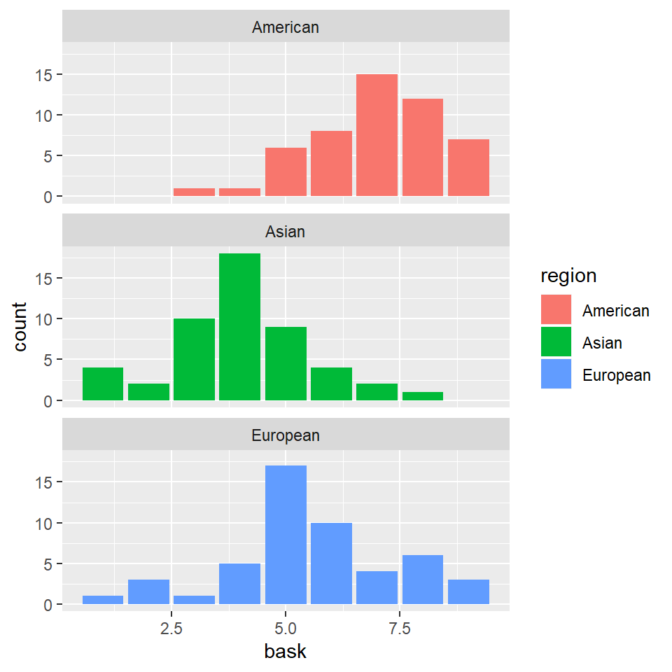
grades %>% ggplot(aes(x = height)) + geom_histogram(aes(fill = region)) + facet_wrap(~region,
    nrow = 3)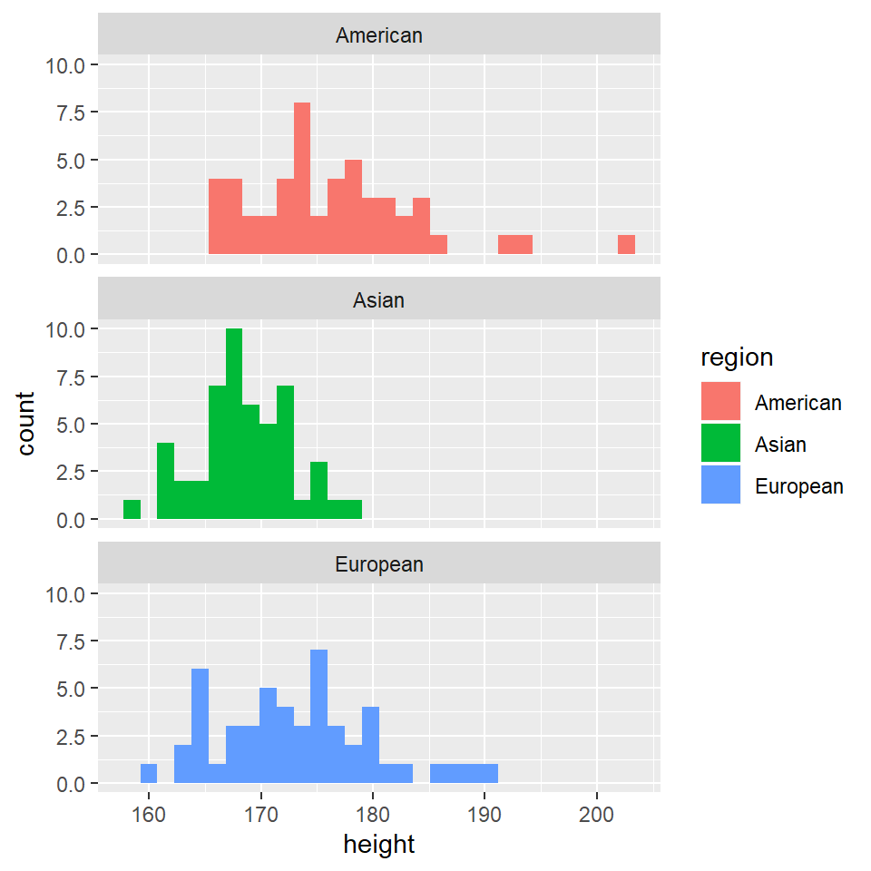
grades %>% ggplot(aes(x = maths)) + geom_histogram(aes(fill = region)) + facet_wrap(~region,
    nrow = 3)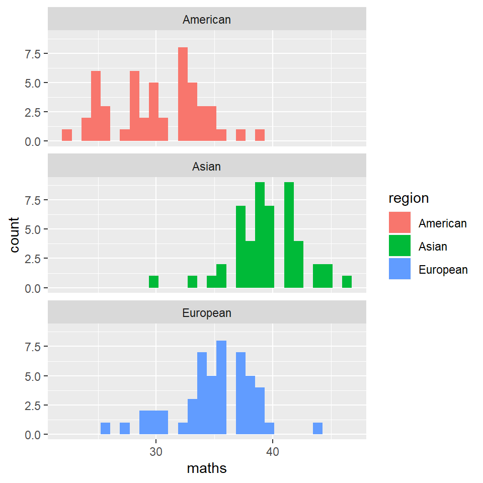
grades %>% ggplot(aes(x = lang)) + geom_histogram(aes(fill = region)) + facet_wrap(~region,
    nrow = 3)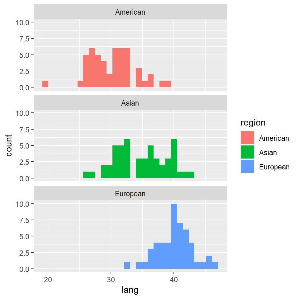
let’s push the envelop a bit… could we spot anything by plotting variables against each other (scatterplot)?
let’s try first with height vs lang
grades %>% ggplot(aes(x = height, y = lang)) + geom_point(aes(color = region))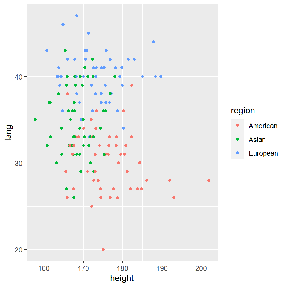
no… cannot see much in the plot above.
how about … maths agains lang
grades %>% ggplot(aes(x = maths, y = lang)) + geom_point(aes(color = region))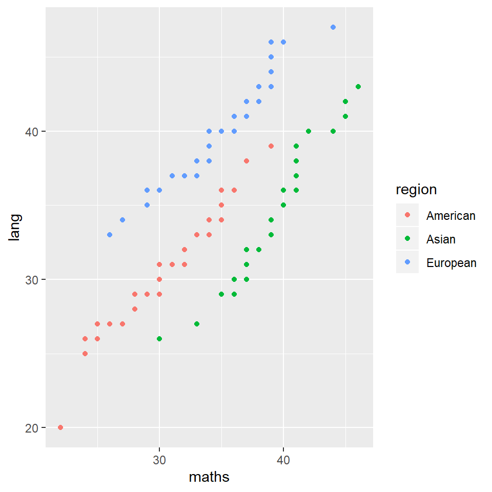
wow, there are some clear patterns there… but what do they mean?
Clearly, we went straight for a separation of the histograms based on region, and skipped all together the histograms for all participants.
However, while apparently benign, these histograms already convey a lot of information. Different averages are immediately apparent for all region-groups for each of the four predictors.
Of course, at this point we don’t know if these difference are statistically significant, or matter in any way.
For that, we’ll need to see the data’s contribution to the outcome/response variable, i.e., the region of origin.
Here’s where the knn, or the kth nearest neighbor algorithm comes into play. It is an algorithm based on measuring Euclidean distances in the feature space. But before entering into details, let’s see it practice.
Data preparation
The point of this algorithm is to learn from our data; remember, machine learning? It is tempting, therefore, to feed it as much data as we have; after all, the more you get informed, the more you learn, right?
Kind of, but not entirely true, and also, completely forbidden in machine learning. We need to set aside some (part of) data, to validate our results.
First, let’s make sure the data is randomly shuffled.
grades %>% head()## height bask maths lang region
## 1 186.11 7 28 28 American
## 2 178.16 8 36 41 European
## 3 171.16 5 42 40 Asian
## 4 175.55 1 34 39 European
## 5 167.83 6 38 42 European
## 6 168.37 8 34 38 European
which, it appears to be; see how the region entries appear random? But, in case it isn’t, shuffle your data.
# NOT RUN unless you need to (if you loaded my data, it should be randomized by
# rows)
grades <- grades[sample(nrow(grades)), ]  # using base
grades <- slice(grades, sample(1:n()))  # using tidyverse's dplyr
We now need to split our data file into one training and one test data files. There are several ways of accomplishing that, but we’ll go with the simplest one, i.e., we’ll create a vector that we’ll be using as a index to point out certain rows in our original data file. This vector will select randomly a number of rows from our original data file. Again, the number of rows (or the proportion of split) varies, but in our case, we’ll go 2/3 (i.e., 67%) from the original data file for the training data file and 1/3 for the test data file.
# create random selection vector
set.seed(123)
randselect <- sample(1:nrow(grades), 0.67 * nrow(grades))
and only now are we able to effectively split the original data file
# create the training data file
train_grades <- grades[randselect, ]

# create the test data file
test_grades <- grades[-randselect, ]
We’ll also be needing the outcome columns for each our new data file
# labels/records for the outcome feature / response variable in the training data
# file
train_grades_outcome <- train_grades[, 5]

# labels/records for the outcome feature / response variable in the test data
# file
test_grades_outcome <- test_grades[, 5]
and one more step, and we’re ready to put our knn algorithm to good use. Remember that when splitting the data file, we kept the outcome feature (or response variable). But, when running the knn algorithm, we want it to learn from our predictors, not from the labels/outcomes that we want it to predict. Therefore, we need to discard the outcome/response variable, from our input data files, before running the algorithm.
# keep only predictors in the training data file
train_grades_predictors <- train_grades[, -5]

# keep only predictors in the test data file
test_grades_predictors <- test_grades[, -5]
Algorithm implementation
And, here we are, finally ready to run our knn algorithm. It has only one line, but it does so much.
# running the knn algorithm
grades_prediction <- knn(train = train_grades_predictors, test = test_grades_predictors,
    cl = train_grades_outcome, k = 3)
If you run grades_prediction separately, you’ll see it’s a vector containing labels corresponding to the outcome/response variable, and its length equal to the length of the test set.
# summary of prediction
grades_prediction %>% summary
## American Asian European
## 16 19 15grades_prediction %>% length## [1] 50
That’s good! That’s actually great. Our knn algorithm performed exactly as expected. It ‘studied’ the training data set, it learned from comparing its features (remember that data set contained only predictors) with the training outcome set (see the ‘cl’ classifier provided), and it yielded as response a vector corresponding to our test data set.
The only thing left for us to do now is to see how well it performed. For that, we need to contrast the predictions with the actual values corresponding to our test data set. And for that, we’ll be using what’s called a “confusion table”, which matches the number of correct/actual values with the predicted values.
However, just eyeballing the confusion table is not enough to give us a measure of how well our knn model performed. For that, we’ll need to compute the accuracy.
# confusion table
confusion_table <- table(grades_prediction, test_grades_outcome)

confusion_table
## test_grades_outcome
## grades_prediction American Asian European
## American 16 0 0
## Asian 0 19 0
## European 0 0 15# computing the accuracy, as the ration between correctly identified responses
# and total number of responses
grades_fit_accuracy <- sum(diag(confusion_table))/sum(confusion_table)
grades_fit_accuracy## [1] 1And here we are, predicting with 90% accuracy the region of origin of the students that enroll in our university, if we use their sport habits, like the frequency of playing basketball, some data about their physical makeup, like their height, and their academic performance, like scores in maths and knowledge of a second language.
Note: there are other metrics to be considered for the model fit, but we’ll get to them later.
Task requirement #2
What if scenario 1 was different? What if, instead of asking us to predict the students’ nationality or origin, the school had asked to use the origin of the students, together with the other two predictors, knowledge of a second language, and frequency of playing basketball, to forecast their performance in maths (which stands here for the academic performance)? Would we be able to do that?
Hint: the classical statistics tells us we should be able to do it, since being a predictor doesn’t imply causality, but only association.
Solving task #2
Before attempting to solve task # 2, there are a couple of changes, or better said, transformations, that we need to make to our data. Since K-nn is a classifying algorithm, we would need the academic performance to be transformed from a numeric variable expressed as discrete scores in the interval 0-50 into a categorical variable, with say, three levels, like “low proficiency”, “medium proficiency”, and “high proficiency”.
However, a word of caution is important here. Remember we used numerical predictors, so we’ll transform our region in a numeric variable, alebit, obviously, very forcesfully so.
# create a new data file, identical with the previous one,
# but with academic performance coded in four successive categories
# lowest = 1:12, low = 13:24, high = 25:37, highest = 38:40
grades_cat <- grades %>%
  mutate(
    mathscat = ifelse(
      maths %in% 0:12,
      "lowest",
      ifelse(
        maths %in% 13:24,
        "low",
        ifelse(
          maths %in% 25:37,
          "high",
          "highest"
        )))) %>%
  mutate(mathscat = as.factor(mathscat)) %>%
  mutate(
    maths=NULL
  ) %>%
  mutate(
    region = ifelse(
      region == "American",
      1,
      ifelse(
        region == "Asian",
        2,
        3
      ))

  )
# get an overview of how many instances in each category for performance in maths
grades_cat$mathscat %>% table()
## .
## high highest low
## 97 50 3# split the data into training and test sets
train_grades_cat <- grades_cat[randselect, ]
test_grades_cat <- grades_cat[-randselect, ]
# identify the position of the outcome in the new files train_grades_cat %>%
# which(mathscat)
# create inputs for training and classifier vector
train_grades_cat_predictors <- train_grades_cat[, -5]
train_grades_cat_outcome <- train_grades_cat[, 5]
test_grades_cat_predictors <- test_grades_cat[, -5]
test_grades_cat_outcome <- test_grades_cat[, 5]
# running knn
grades_pred_cat <- knn(train = train_grades_cat_predictors, test = test_grades_cat_predictors,
cl = train_grades_cat_outcome, k = 3)
# summary of prediction
grades_pred_cat %>% summary## high highest low
## 32 17 1grades_pred_cat %>% length## [1] 50# confusion table
confusion_table_cat <- table(grades_pred_cat, test_grades_cat_outcome)
confusion_table_cat## test_grades_cat_outcome
## grades_pred_cat high highest low
## high 26 6 0
## highest 4 13 0
## low 0 0 1# computing the accuracy, as the ration between correctly identified responses
# and total number of responses
grades_cat_fit_accuracy <- sum(diag(confusion_table_cat))/sum(confusion_table_cat)
grades_cat_fit_accuracy## [1] 0.8Final notes
By now, you’d have realized that there are some very important aspects left to clarify. For instance, how to choose a suitable number of classes. We knew there were three such main groups by region, but what if there is no real clustering beside that.
Or, is there a certain condition as to what type of data befits the knn algorithm, i.e., should we use only certain type of data as predictor features? The answer to these questions, albeit extremely important, of course, is beyond the scope of this particular exercise.
Data normalization
Untill here, since this is more or less a didactic example, and less of a real life scenario, we used the data as it came. However, since knn is based on measuring the Euclidian distance between points in the feature space, it is sensitive to using very different measuring scale (for the predictor variables). As such, data normalization, i.e., bringing all predictors to the same scale of measurement, so that each one contributes equally to the clusters identification, is The normal and usual procedures.
kNN assumes numeric data
kNN benefits from normalized data
- prepare a normalizing function
# define a min-max normalize function
normalize <- function(x) {
    return((x - min(x))/(max(x) - min(x)))
}
A continued analysis or a bit of homework, if you will
We’ve use a very simple line of code to predict students’ region of origin. And, in that line of code, our k of choice was 3, and that’s because it was set for you. But the whole key of the knn algorithm is actually to find the k that gives an optimally sufficient fit to the data. Please, note that I didn’t say “the best” fit, but the optimally sufficient fit.
Hence, it is your turn now to experiment with various k-s and find better fit for your model. Try modifying your k and see what it’ll get you. One last piece of information about k; one commonly encountered suggestion is to use k = sqrt(n), where n is the number of cases/records in your data file.
Also, normalize the data in the predictors’ sets and see if that changes anything.
Remember having “fresh data” for validation
As I said above, it is paramount to have data for validation. What’s also equally important is that these data are not touched in any shape or form before validation. Once you selected that data, you don’t use it for anything else than validate your results.
But, you may wonder with transpiring anxiety, “what if I don’t have enough data, and the little that I use to train my model will leave it dumb?”. Well, again, like with everything else in machine learning, you’ll see that some clever guys devised a way around that.
Also, you’ll see several recommendations for the proportion of split. Some will say 10% vs 90%, others will flush the 80-20 rule, whereas others will graciously explain that the real art lies in splitting 1/3 to 2/3 (the largest part going into the training, whereas the smallest part constitute the test data file).
Again, take everything with a grain of salt and use your own reasoning. What determines the proportion of split? The answer is the need to provide enough data to learn, while balancing it with the need to have (enough) data for validation (think raw numbers here).
Therefore, the rule of thumb is, the larger your data set, the bigger the proportion you can allocate to your training set. Mind the overfit, though (that’s another discussion, for another meeting). In our case, we had only 150 data points and it was crucial to keep enough of them for validation, hence, the choice for the 1/3 vs 2/3 split.
A note about the data
These data are obviously (or perhaps, if I did it right, not very obviously) made up. Perhaps, schools not recording their students heights and basketball habits very often gave it away, or perhaps for those already familiar with knn something looked familiar. At any rate, while realistic enough for our example, the data are not real. For those interested in how it was created, please ask during our meetings.
Last modified on 2021-04-07