lastmod: 11 May, 2020

Preamble - introduction to the problem

Note: This post builds up on a previous post, but it isn’t conditional on that. You can follow it as is, or you can take a look first at the previous post (see below)

In a previous post (“Machine Learning - Supervised Learning - KNN”) we used the knn algorithm to predict class membership for our cases, based on a selection of predictors.
In performing this task, we used k, i.e., the number of neighbors used by the algorithm, and we also knew the categories of our outcome/response variable, which we used to train our model.

However, suppose (for a very convoluted reason that I cannot really fathom on the spot), that we didn’t look at the response variable and we did not know how many categories it is comprised of (remember, American, Asian, and European). Actually, say we didn’t know that there is a response variable in the first place; hence all variable are just some features of a data set…

Would we still be able to conclude that at some level, our data can be segregated into three groups?

Further more, say that even if we knew the region of origin for each participant, it doesn’t necessarily mean there is anything else grouping those participants together. Perhaps, Asian students’ only link/closeness to other Asian students is only in the name of their region of origin, and the same may be true for Europeans and Americans. Do we have any procedure (algorithm) that would look at the other data and find out?

Fortunately, we do. Let’s try to find the answer to that using a procedure called hierarchical clustering. Well, this is actually the ‘umbrella’ term for a family of procedures.

Solution

First, let’s equip ourselves with the required libraries.

# libraries
library(tidyverse)  # data manipulation
library(cluster)    # clustering algorithms
library(factoextra) # clustering visualization
library(dendextend) # for comparing two dendrograms

Second, let’s prepare our data (if you need to reload it, you can download it from here).

# read in the data
grades <- read.csv("https://learning-analytics.dorinstanciu.com/post/ml-knn/_data/knn-grades/grades-sim.csv")
grades %>% head()

##   height bask maths lang   region
## 1 186.11    7    28   28 American
## 2 178.16    8    36   41 European
## 3 171.16    5    42   40    Asian
## 4 175.55    1    34   39 European
## 5 167.83    6    38   42 European
## 6 168.37    8    34   38 European

# create a vector of names for each respondent/case to ease the identification later in dendogram
# create a new column based on the region and row number
grades <- grades %>% 
  mutate(
    id=row_number()
  ) %>% 
  mutate(id=str_c(region,"_",id))

# create the vector of names
rownames_grades <- grades$id

# nullify the column of names
grades <- grades %>% 
  mutate(id=NULL)

# normalize the data
grades_norm <- grades %>% 
  mutate(region = ifelse(region == "American",
                         1, 
                         ifelse(region=="Asian", 2,3))) %>% 
  scale()

# set rownames for the normalized data
rownames(grades_norm) <- rownames_grades

grades_norm %>% head()

##                height       bask      maths       lang    region
## American_1  1.8900509  0.7415944 -1.3337585 -1.3166589 -1.220656
## European_2  0.7719633  1.2426717  0.2201349  1.1032137  1.220656
## Asian_3    -0.2125163 -0.2605602  1.3855550  0.9170697  0.000000
## European_4  0.4048930 -2.2648694 -0.1683385  0.7309256  1.220656
## European_5 -0.6808474  0.2405171  0.6086083  1.2893577  1.220656
## European_6 -0.6049018  1.2426717 -0.1683385  0.5447816  1.220656

Aglomerative hierarchical clustering (AGNES)

The name AGNES stands for agglomerative nesting. This is a bottom-up procedures, in that it starts with each item being compared against the others, and being paired up with the most similar. Each step brings more and more items together until all items are combined into a single cluster, or, because the whole process resembles a tree, until the root is found.

hclust function

# Agglomerative clustering using hclust 

# dissimilarity matrix

dissim_grades_norm <- dist(grades_norm, method = "euclidian")

# hierarchical clustering using hclust (complete linkage)
hcl_grades_norm <- hclust(dissim_grades_norm, method = "complete")

# Plot the dendogram
plot(hcl_grades_norm, cex = 0.6, hang = 0.3, xlab = "respondents")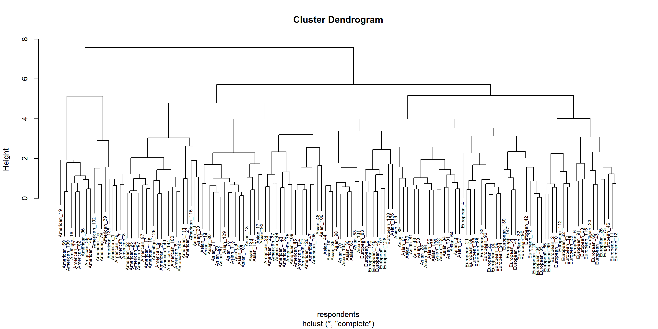

using AGNES

We’ll demonstrate the bottom up aglomerative clustering using agnes(), as alternative to hclust() before. This time, we’ll even get several fit indices to compare, for each method.

# aglomerative clustering using agnes

# methods to assess

listofmethods <- c( "average", "single", "complete", "ward")
names(listofmethods) <- c( "average", "single", "complete", "ward")

# function to compute coefficient
aglclust <- function(x) {
  agnes(grades_norm, method = x)$ac
}

map_dbl(listofmethods, aglclust) %>% round(3)

##  average   single complete     ward 
##    0.871    0.624    0.914    0.973

##   average    single  complete      ward 
## 0.7379371 0.6276128 0.8531583 0.9346210

acl_grades_norm <- agnes(grades_norm, method = "ward")
pltree(acl_grades_norm, cex = 0.6, hang = .3, main = "Dendogram using AGNES" )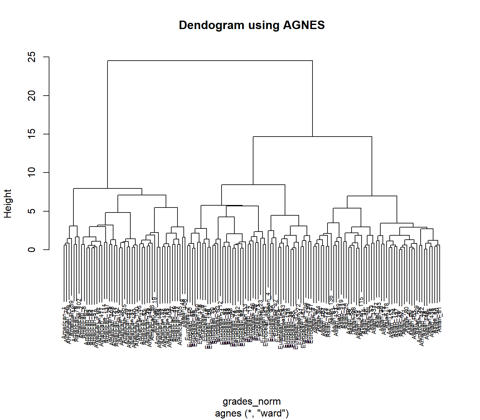

Divisive hierarchical clustering (DIANA)

The divisive hierarchical clustering (DIANA is the short name for Divisive Analysis) works in a top-down order, hence, the oposite of AGNES. It begins with the root, which includes all cases in a single group/cluster. The process goes iteratively towards the bottom, separating items at each step based on their similarity, or dissimilarity, for that matter. The difference between AGNES and the previous, top-down algorithms, is that there is no method for AGNES.

# compute divisive hierarchical clustering
dcl_grades_norm <- diana(grades_norm)

# Divise coefficient; amount of clustering structure found
dcl_grades_norm$dc %>% round(3)

## [1] 0.902

## [1] 0.8514345

# plot dendrogram
pltree(dcl_grades_norm, cex = 0.6, hang = 0.3, main = "Dendrogram of diana")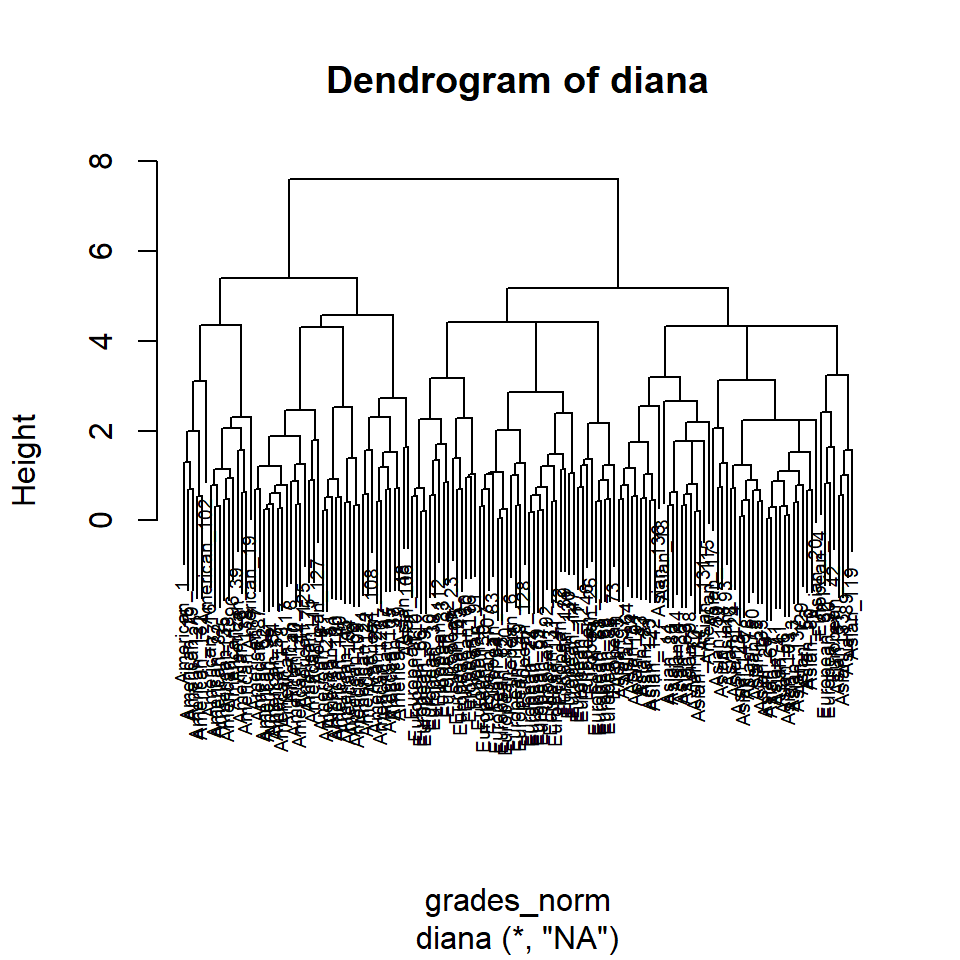

Conclusions

The comparison of the dendograms provided by hclust() and, respectively diana() reveals two rather different solutions. The first seems to indicate a 3-cluster solution whereas the latter suggests a 4-cluster solution. Since the data aglomeration is a mathematical construct, it is up to the researcher to identify dogmatic/theoretic reasons to support these assertions and, if necessary, to investigate further using procedures like latent class or latent profile analysis.